Homework
5 (due 2/25)
CSC 431
This week we finished chapter 3 (3.2, 3.3, very superficially, and some of 3.4; we did not cover any of the particular orthogonalization methods in 3.5, but talked about SVVD decomposition in 3.6). After that we continued on to non-linear systems in chapter 5, covering material in sections 5.1 -5.4 and 5.5.1, 5.5.2.
During class we saw some of Heath's simulations:
and we discussed my solutions to homework 4,
problem 4 and problem 5 and programs
illustrating svd and
pseudoinverse.
Submission: you can submit the homework by hardcopy in class or by sending it to me as an email.
Note: for all of the problems on this homework you can use the computer, but still explain your steps.
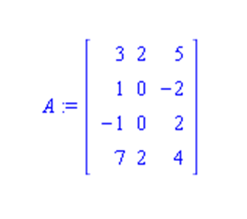
1. [Projectors, 20pt] (You are given the matrix

a) Determine the projector P onto span(A).
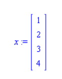
b) For the vector x

determine the closest vector x' in span(A), by using the projector. Also compute the Euclidean distance between x and x'.
c) For the matrix A from part a) find a vector b that is close to being orthogonal to span(A). Use that vector b and several small perturbations of it to solve the system Ax = b (using the comptuer). Compare the relative change of b with the relative change of x.
2. [Data fitting, 15pt] You are observing a time series whose behavior seems to match a model of the form f(x) = a sin(x) + b x + c with unknown parameters a, b, and c. You've experimentally observed the following data:
| x | f(x) |
| 1.0 | 9.9 |
| 1.1 | 10.8 |
| 2.4 | 12.0 |
| 2.9 | 7.8 |
| 3.1 | 5.9 |
| 8.2 | 32.9 |
Determine a, b, and c for a linear least square fit to this data.
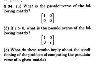
3. [Pseudoinverse, 10pt] Do Exercise 3.34 of the book (page 152) on computing pseudoinverses of small matrices:

4. [Fixed Points, 10pt] Do Exercise 5.6, parts a) and b) (page 249 of the book, page 176 in the first edition).
Marcus SchaeferLast updated: February 19th, 2010.